
I already wrote a paper called “Lill’s Method and Graphical Solutions to Quadratic Equations” that shows how to solve quadratic equations using Lill’s method. In this post I want to show an alternative way of solving quadratic equations that have complex or imaginary roots. This method was briefly mentioned in the paper “Geometric Solution of the Quadratic Equation” by G.A. Miller [1].
If you are not familiar with Lill’s method, you can read this article by Verner Bradford and other articles linked on this page. There are more than one way of illustrating a polynomial using Lill’s method, but Bradford’s way is the most convenient.
Quadratic With Complex Roots
I will illustrate the method with a specific quadratic of the form ax2 +bx +c=0 that has complex roots. A good example is x2 +2x + 5=0, since the roots are x1 = 1 – 2i and x2 = 1 +2i. Thus the polynomial has the coefficients a=1, b=2 and c=5.
The Lill representation of x2 +2x + 5=0 can be seen below. Again, I used Bradford’s way of representing the polynomial. This is the most useful and convenient method since it always has the point P1 at (0,0). P0 and P1 are the points that make the segment that corresponds to the coefficient a=1. P1 and P2 make the segment for b=2, and P2 and P3 make the segment for c=5. It’s easy to see that the length of the segments are equal to the absolute value of the coefficients (in our case all the coefficients are positive).

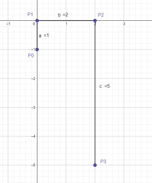
People that want to understand the orientation of the segments can use the method explained by Bradford. I prefer to look in terms of counterclockwise or clockwise rotation. If the coefficients a and b have the same sign, then the segment corresponding to b is rotated 90 degrees counterclockwise with respect to the segment a. In our case, both coefficients are positive so the segment b is 90 degrees counterclockwise with respect to a (segment a points North, while segment b points East). The coefficients b and c also have the same sign, so segment c points 90 degrees counterclockwise with respect to segment b (c points South).
Lill Circle
In my old article I showed how to use the Lill circle to find the roots of a quadratic with real coefficients. You can also use the Lill circle to find the complex roots of a quadratic equation.
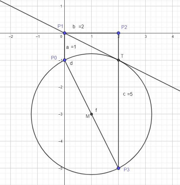
To construct the Lill circle, you simply create the circle who’s diameter is P0P3. The next step is to create the 2 tangents from the point P1 to the Lill circle (one tangent is enough). In the image below, point T is the intersection point between the Lill circle and one of the tangents from point P1.

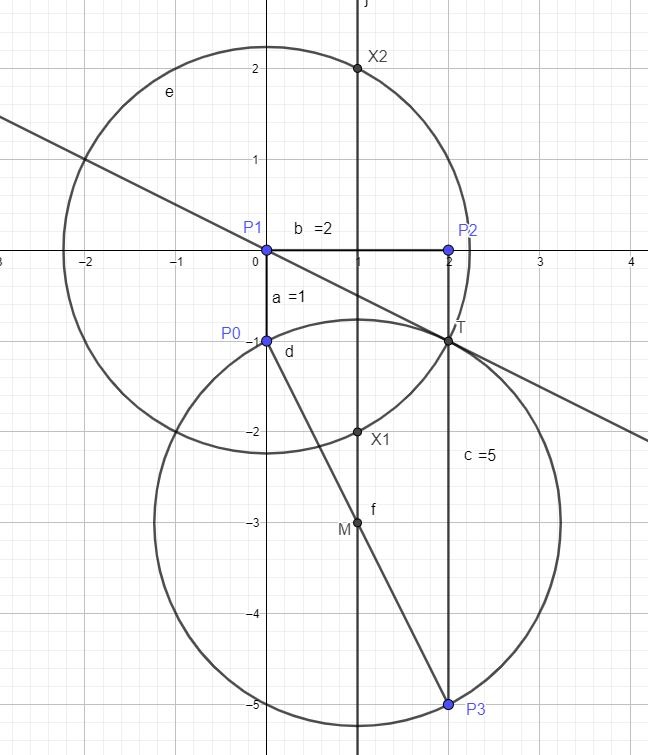
The next step is to create the perpendicular to the segment b from M (the center of Lill’s circle). An alternative is to construct the perpendicular bisector of the segment b. The points X1 and X2 that correspond to the 2 roots, are the points of intersection between the perpendicular bisector and the circle with center at P1 and radius equale to P1T. The coordinates of X1 are (1,-2) and the coordinates of X2 are (1,2). This solves our equation since x1 = 1 – 2i and x2 = 1 +2i (x coordinate gives the real part and the y coordinate gives the complex or imaginary part).

Final Notes
In my old paper I mentioned that the coefficient a works as a scale factor. If a doesn’t have an absolute value of 1, than you need to divide by the absolute value of a to obtain the value of roots from the coordinates of points X1 and X2. For example, you can try to solve the polynomial 2x2 +4x + 10=0 using the technique described above. The polynomial has the same roots as our example (all the coefficients were multiplied by 2). However, the coordinates of the points X1 and X2 are going to be (2, -4) and (2, 4). You have to divide all the coordinate numbers by abs(a)=2 to obtain the value of the roots.
In my old paper I also mentioned without proof that the point X1 is the inverse of point X2 with respect to the Lill circle (You can learn about inversive geometry on this Wikipedia page). I think that I am the first person who wrote about this circle inversion property of the Lill circle. Maybe in the future I will try to do an actual proof of the property. If the property is true, it shows the beauty of Lill’s method and the usefulness of Lill circle. There are probably other interesting properties that were not discovered.
For more articles about Lill’s method check this resource page and also check my articles.
Sources
[1] Miller, G. (1925). Geometric Solution of the Quadratic Equation. The Mathematical Gazette, 12(179), 500-501. doi:10.2307/3602823
2 comments